The purpose of this project is to study nuclear reactors in Japan. First we’ll read in the required libraries.

library(dplyr)
library(knitr)
library(ggplot2)
library(rvest)
library(lubridate)
library(scales)

Now we will read in tables of nuclear reactors from Wikipedia http://en.wikipedia.org/wiki/List_of_nuclear_reactors via the webscraping library, rvest.

page <- "http://en.wikipedia.org/wiki/List_of_nuclear_reactors"
table_nodes <- page %>%
  read_html() %>%
  html_nodes("table")
table_list <-
  html_table(table_nodes[1:30], fill = TRUE)

After some searching, we find the relevant table is at position 25.

table <- table_list[[25]]
table %>% head() %>% kable()

Name Unit No. Reactor Reactor Status Capacity in MW Capacity in MW Construction Start Date Commercial Operation Date Closure
—————— ——— ——– ——– ———————- ————— ————— ———————— ————————– —————– Name Unit No. Type Reactor Model Capacity in MW Capacity in MW Construction Start Date Net Gross
Fukushima Daiichi 1 BWR BWR-3 Inoperable 439 460 25 July 1967 26 March 1971 19 May 2011
Fukushima Daiichi 2 BWR BWR-4 Inoperable 760 784 9 June 1969 18 July 1974 19 May 2011
Fukushima Daiichi 3 BWR BWR-4 Inoperable 760 784 28 December 1970 27 March 1976 19 May 2011
Fukushima Daiichi 4 BWR BWR-4 Shut down/ Inoperable 760 784 12 February 1973 12 October 1978 19 May 2011
Fukushima Daiichi 5 BWR BWR-4 Shut down 760 784 22 May 1972 18 April 1978 17 December 2013

Now we fix the column names.

names(table) <- c("Name",   "Reactor_No", "Type", "Model", "Status", "Net_Capacity", "Gross_Capacity", "Construction_Start_Date", "Commercial_Operation_Date", "Closure")
table <- table[-1, ] # drop the first row

Now we use lubridate to make genuine date columns.

table <- table %>% mutate(Construction_Start_Date = parse_date_time(Construction_Start_Date, "dmy"),
                          Commercial_Operation_Date = parse_date_time(Commercial_Operation_Date, "dmy"),
                          Closure = parse_date_time(Closure, "dmy"))

Now we plot the construction start date versus the net capacity and type.

table  %>% filter(Type != "") %>% 
  ggplot(aes(x = Construction_Start_Date, y = Net_Capacity)) +
  geom_point(aes(color = Type)) +
  labs(x = "Construction Start Date", y = "Net Capacity")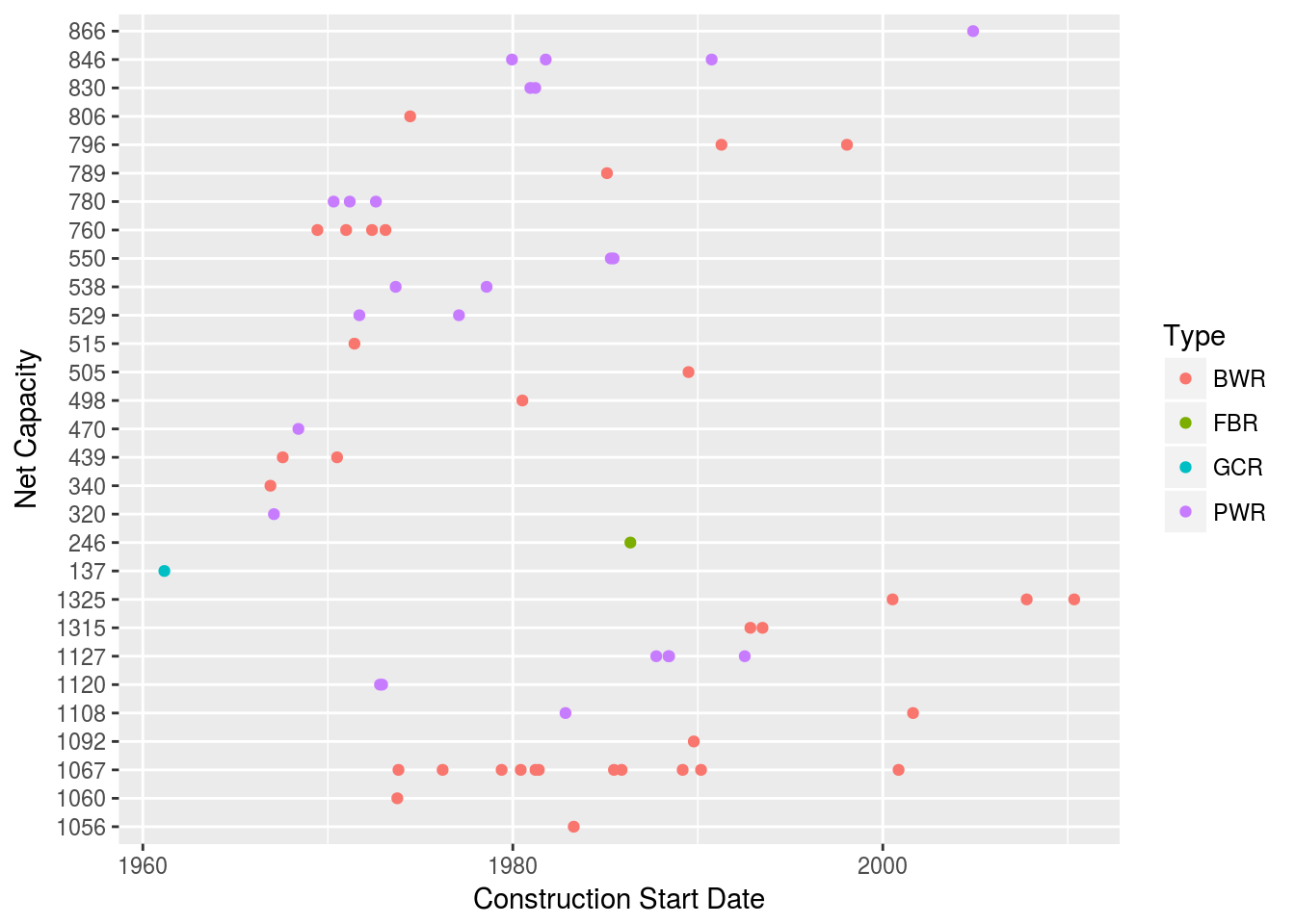

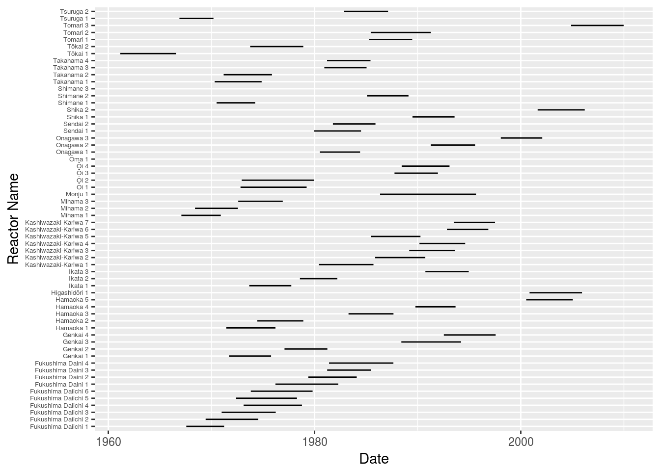
Finally we make an informative graphic that shows how long it took between start of construction and commissioning for each nuclear reactor.

table$num <- 1:nrow(table)

table  %>% filter(Type != "") %>%
  mutate(Name = paste(Name, Reactor_No)) %>%
  ggplot(aes(y = num)) +
  geom_segment(aes(x = Construction_Start_Date, y = Name, xend = Commercial_Operation_Date, yend = Name)) +
  theme(axis.text.y=element_text(size=5)) +
  labs(x = "Date", y = "Reactor Name")