Housing Prices
Oliver Thistlethwaite
In this project, we will analyze house prices from Saratoga, CA.
First we will read in the required libraries and a database of house prices.
library(dplyr)
library(readr)
library(ggplot2)
library(knitr)
library(caret)

houses = read_csv("http://tiny.cc/mosaic/SaratogaHouses.csv")
houses %>% head() %>% kable() | Price | Living.Area | Baths | Bedrooms | Fireplace | Acres | Age |
|---|---|---|---|---|---|---|
| 142212 | 1982 | 1.0 | 3 | N | 2.00 | 133 |
| 134865 | 1676 | 1.5 | 3 | Y | 0.38 | 14 |
| 118007 | 1694 | 2.0 | 3 | Y | 0.96 | 15 |
| 138297 | 1800 | 1.0 | 2 | Y | 0.48 | 49 |
| 129470 | 2088 | 1.0 | 3 | Y | 1.84 | 29 |
| 206512 | 1456 | 2.0 | 3 | N | 0.98 | 10 |
From examining the head of the file, we see what information the database provides us.
Next we will convert all the columns into numeric data.
houses <- houses %>% mutate(Fireplace = ifelse(Fireplace == "N",0,1))Next we will create a training set and testing set to test some machine learning algorithms. We’ll use 80% of the data for training and 20% for testing.
set.seed(3)

index <- 1:nrow(houses)
testindex <- sample(index, trunc(length(index)/5))

train <- na.omit(houses[-testindex,])

test <- na.omit(houses[testindex,])
testsize <- nrow(test)
We’ll compare the different models by mean squared error. First we’ll try the NULL Model (The model whose output is always the mean of the output variable).
mod <- lm(Price ~ 1, data = train)

pred <- predict(mod, test)

mse <- sum( ( pred - test$Price )^2 ) / testsize

mse^(1/2)
## [1] 99636.08So on average our error is about $100,000 which is unacceptable.
Next we’ll try a linear model.
mod <- lm(Price ~ ., data = train)

pred <- predict(mod, test)

mse <- sum( ( pred - test$Price )^2 ) / testsize

mse^(1/2)
## [1] 57189.04This is significantly better.
Now we’ll try a Conditional Inference Tree.
mod <- train(Price ~ ., data = train, method = "ctree")

pred <- predict(mod, test)

mse <- sum( ( pred - test$Price )^2 ) / testsize

mse^(1/2)
## [1] 63163.48More or less the same as the linear model. Finally we will plot the resulting model.
plot(mod$finalModel)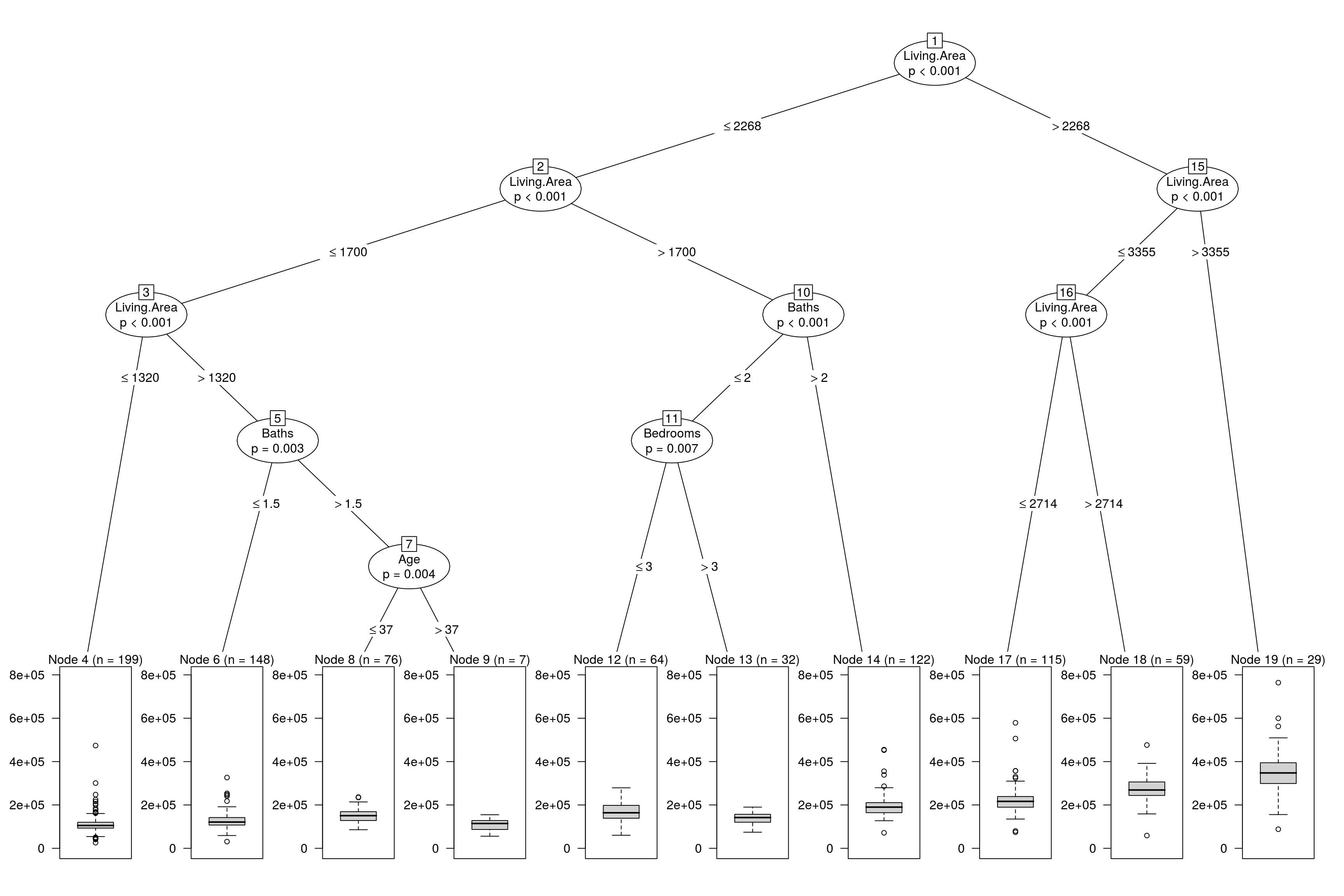
Principal Component Analysis
Finally we’ll try to apply PCA (principal component analysis) and see if that improved our results. First we will create the principal components using the feature columns.
prin_comp <- prcomp(train %>% select(-Price), scale. = T)

std_dev <- prin_comp$sdev
pr_var <- std_dev^2
prop_varex <- pr_var/sum(pr_var)
Next we will examine the cumulative proportion of variance explained for the principal components.
plot(cumsum(prop_varex), xlab = "Principal Component",
              ylab = "Cumulative Proportion of Variance Explained",
              type = "b")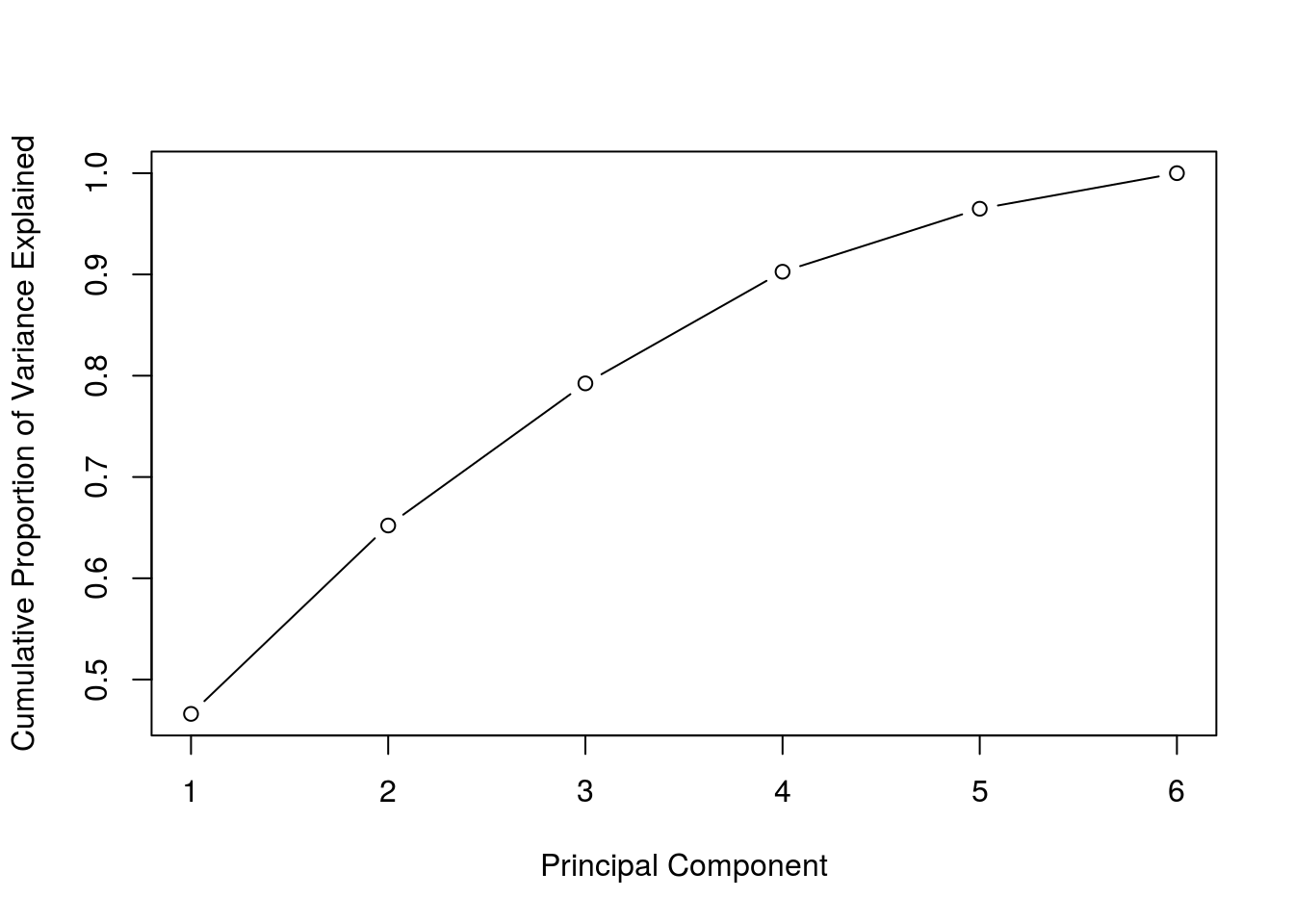
Most of the variance is explained by the first two components. Next we will plot the resultant first two principal components.
biplot(prin_comp, scale = 0)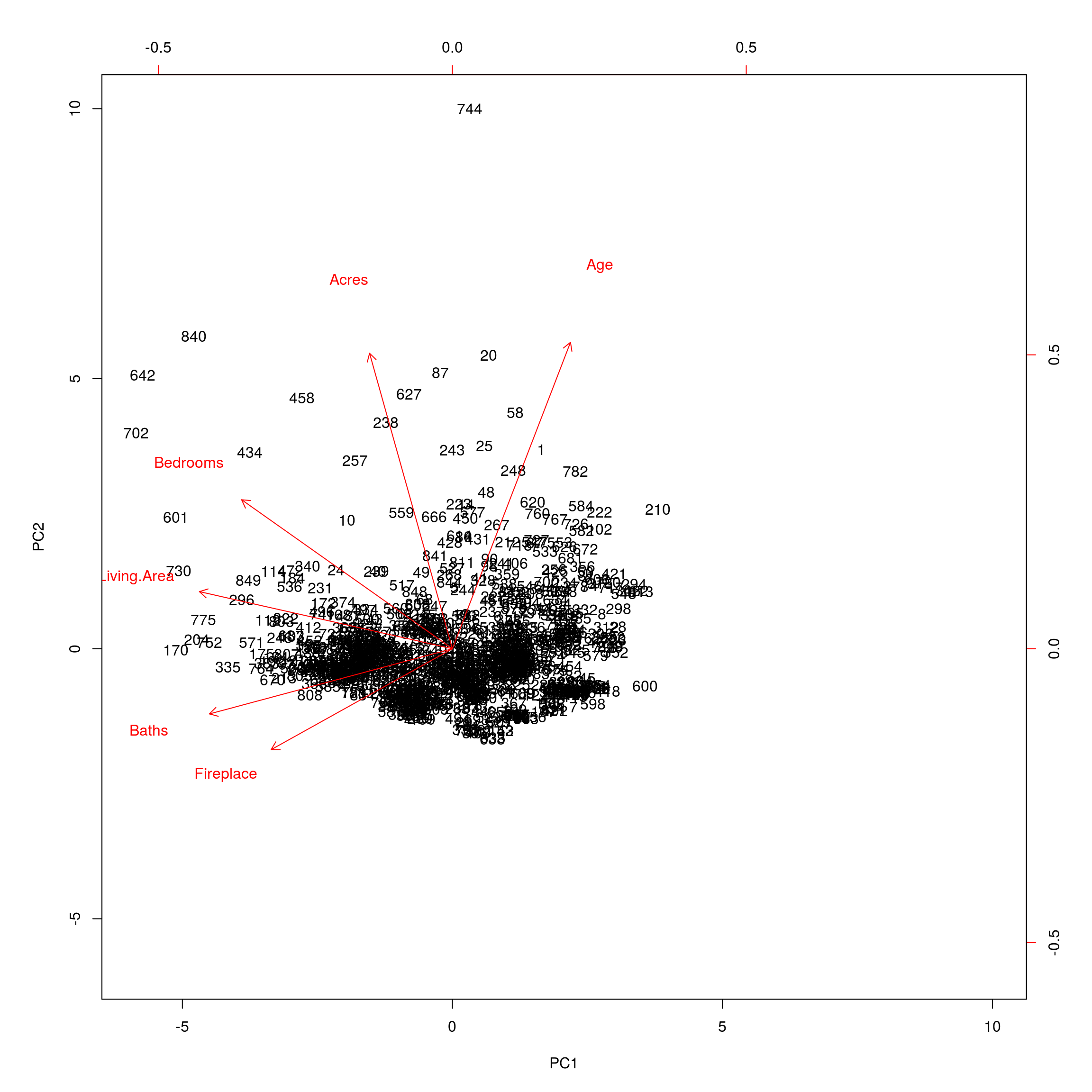
Now to apply some machine learning algorithms, we creat PCA training and testing sets.
train.pca <- data.frame(Price = train$Price, prin_comp$x)

test.pca <- as.data.frame( predict(prin_comp, newdata = test %>% select(-Price)) )
test.pca$Price <- test$Price
Applying a linear model to just the first principal component produces the best mean squared error.
mod <- lm(Price ~ PC1, data = train.pca)

pred <- predict(mod, test.pca)

mse <- sum( ( pred - test.pca$Price )^2 ) / testsize

mse^(1/2)
## [1] 63778.04Observe even though we failed to improve the mean squared error, we did manage to reduce the problem from 6 dimensions to 1 dimension and obtain a similar mean squared error.