The purpose of this project is apply clustering techniques to genetic data. First we read in the required libraries.

library(dplyr)
library(knitr)
library(ggplot2)
library(DataComputing)
library(tidyr)
library(ggdendro)

First we read in the table NCI60 from the DataComputing library. Each row of this time is a genetic probe with the first column identifing the probe and the next 60 correspond to cell lines and their reported expression in each probe. We first convert the table to a narrow format where each row is an individual observation about a cell line in a probe.

Narrow <- 
  NCI60 %>%
  gather(value=expression, key=cellLine, -Probe) %>%
  group_by(Probe, cellLine) %>%
  summarise(expression = mean(expression)) %>% 
  ungroup()

Next we will analyze the standard deviation of the expression numbers for each probe. We also test the Null Hypothesis that there is no relationship between probes and the standard deviations of the expression numbers for each probe.

keep <- 500
Best <-
  Narrow %>%
  group_by(Probe) %>%
  summarise(spread = sd(expression)) %>%
  arrange(desc(spread)) %>%
  mutate(i = row_number()) %>%
  head(keep)

Randomized <-
  Narrow %>%
  mutate(Probe = sample(Probe)) %>%
  group_by(Probe) %>%
  summarise(spread = sd(expression)) %>%
  arrange(desc(spread)) %>%
  mutate(i = row_number()) %>%
  head(keep)

Best %>% 
  ggplot(aes(x=i, y=spread)) + 
  geom_line() +
  geom_line(data=Randomized, color="red", size=1, alpha=.5)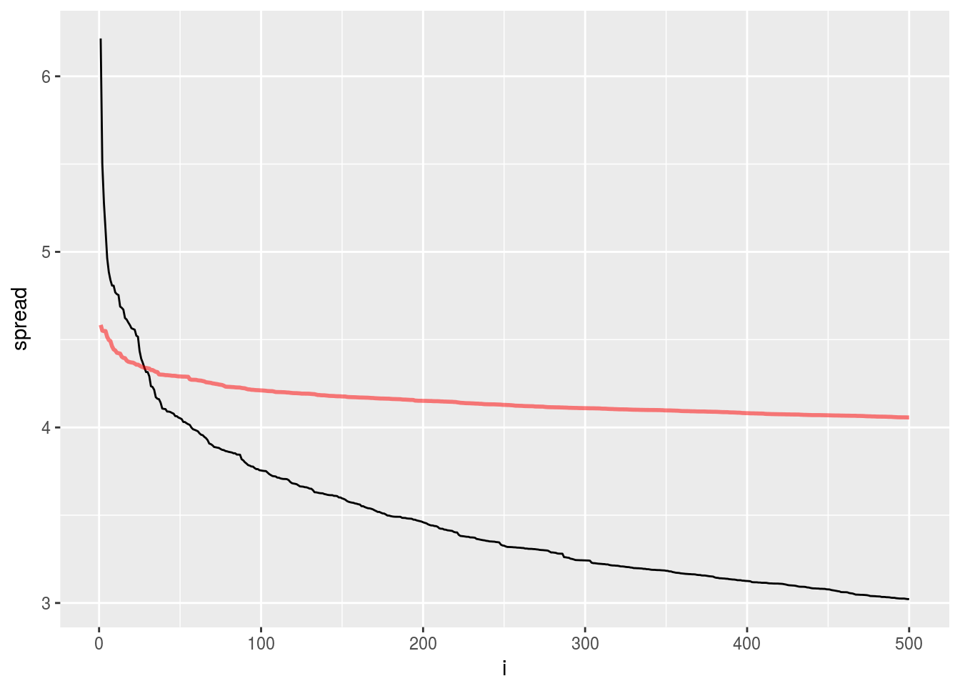

As we can see from there graph, there is clearly a relationship so the Null Hypothesis fails.

Now we filter out those probes with standard deviations of expression numbers that are above a threshold of 4.5.

Keepers <-
  Narrow %>% group_by(Probe) %>%
  filter(sd(expression) > 4.5)

Now we convert the data to a wide format where each row is a cell line and the columns are expression numbers reported by different probes.

Keepers_wide <-
  Keepers %>%
  spread(key=Probe, value=expression)

rownames(Keepers_wide) <-Keepers_wide$cellLine
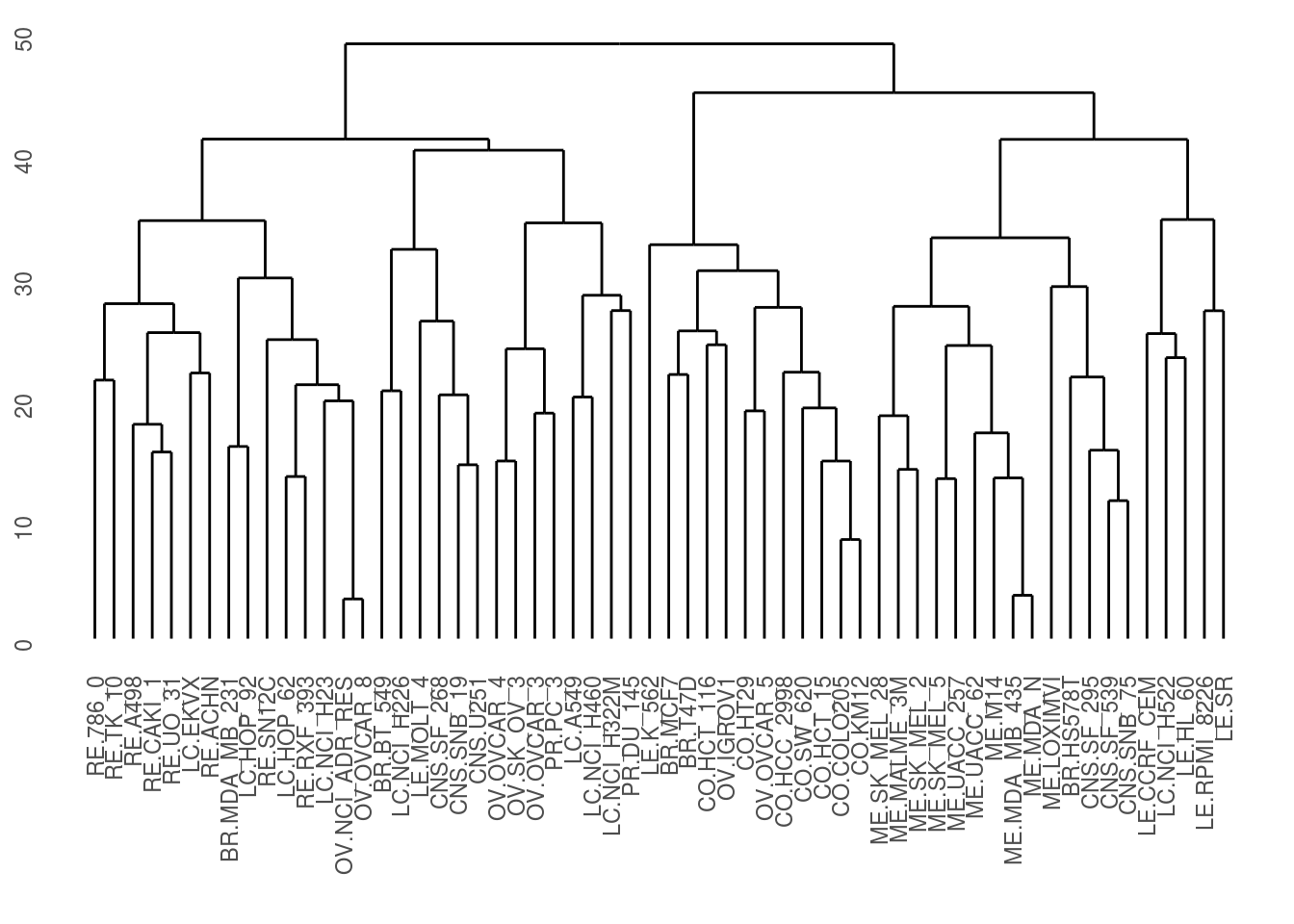
Keepers_wide <- Keepers_wide %>% select(-cellLine)

Now we finally apply a clustering algorithm to make a dendrogram.

Dists <- dist(Keepers_wide)
Dendrogram <- hclust(Dists)
ddata <- dendro_data(Dendrogram)

ggdendrogram(Dendrogram)